Tokenomics series: Projecting the total supply of ICP

[bjoernek]

TL;DR

The goal of this article is to explain the interplay between the deflationary and inflationary mechanisms of ICP and to project their joint development. The concepts and tools presented here serve as a toolbox for assessing ICP tokenomics over time and potential changes.

We have constructed a projection model that considers the development of cycles burned, voting rewards, and node provider rewards to analyze the evolution of the total supply of ICP and maturity. The model is based on historical data and provides insights into the future trends. In an upcoming article, we will conduct scenario analysis to explore the sensitivity of the results to key parameters used in the projection.

According to our model:

• The ICP equivalent of cycles burned is projected to surpass node provider rewards in a little over three years, indicating that the revenue generated by the Internet Computer will exceed operational costs.
• In five to six years, the ICP equivalent of cycles burned is predicted to surpass the combined sum of node provider rewards and voting rewards, resulting in deflationary conditions.

This article is the second installment in our tokenomics series. In the first piece, we focused on projecting cycle demand and the necessary network capacity. If you have not read it yet or need a refresher, you can find it here.

Recap on NNS rewards

The Internet Computer (IC) has inflationary and deflationary mechanisms. Governance participants can convert voting rewards to newly minted ICP. Also, node providers receive rewards in the form of newly minted ICP tokens. On the other hand, ICP is converted to cycles (i.e., burned) in order to pay for computation and storage. The diagram below illustrates this process.

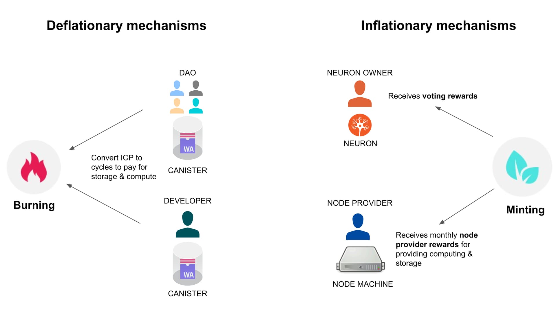
Voting rewards

The NNS serves as the decentralized autonomous organization (DAO) that governs the Internet Computer. Decisions are made in the NNS via voting, where token holders who have staked ICP in “neurons” can vote. Each day a voting reward pool is allocated to the voting neurons in the NNS. Each neuron receives a proportional share of the reward pool, determined by its respective voting power and the number of proposals in which it participated. Here’s a detailed explanation of how this process works:

Determination of the total reward pool

• For a given time period, t, ranging from the genesis time (G) to G + 8 years (8y), the annualized reward as a percentage of the total supply is calculated using the formula: R(t) = 5% + 5% [(G + 8y – t)/8y]². For any time t after G + 8y, the reward percentage is a fixed 5%: R(t) = 5%. The voting rewards function on the dashboard visualizes the annualized voting reward allocation.
• The total pool of voting rewards for a particular day is determined by multiplying the ICP supply (total supply of ICP tokens on that day) with R(t) and then dividing by 365.25.
• For example, on April 10th, 2023, the total supply of ICP was 497.4M tokens. The voting reward function for that day was calculated as 7.89%, leading to a total pool of voting rewards amounting to 107K.

Voting power of neurons

• Only neurons with a dissolve delay of more than 6 months are eligible for voting, and the maximum dissolve delay is 8 years.
• The voting power of a neuron is calculated as the product of the neuron’s stake, the dissolve delay bonus, and the age bonus.

Allocation of reward pool to neurons

The reward pool is distributed proportionally based on the voting power of settled proposals for that day, multiplied by the reward weight of the respective proposal category.

• The set of proposals included in the reward period (usually a day) consists of proposals that are no longer open for voting and have not yet settled in terms of voting rewards.
• The total voting power of eligible neurons is aggregated.
• Each neuron is rewarded according to the proportion of its voting power contributed to these proposals, multiplied by the reward weight of the corresponding proposal category.

When a neuron receives voting rewards, they are recorded as maturity, which is an attribute of the neuron and not a tradable asset. If a user wishes to convert maturity into ICP, they must burn the maturity by spawning a new neuron, which is a non-deterministic process described in detail here.

Node provider rewards

Node provider rewards are paid out in the form of newly minted ICP tokens and are calculated on a monthly basis for each individual node. The reward amount per node depends on two factors: the node’s location, as hosting prices may vary across different locations, and the type of node, determined by its hardware specifications and connectivity capabilities.

To account for the investment and operational costs incurred by node providers, which are typically denominated in fiat currency, the node provider rewards are specified in Special Drawing Rights SDR (currency code XDR), which represents a basket of fiat currencies consisting of USD, EUR, RMB, YEN and GBP. These rewards are then converted into ICP tokens using the average exchange rate over the previous 30 days. For example, in April 2023, the total amount of ICP paid out as node provider rewards was 363K.

Projection model

In this section, we describe the joint simulation of cycles burned, voting rewards, and node provider rewards. By doing so, we can also simulate the development of the total ICP supply and maturity. For this analysis, the underlying period for simulation steps is set to one month.

Inputs to the calculation

Supply parameters as per April, 10th ‘23

• Total supply of ICP at the specified date: ICP_total_supply[0] = 497.4M.
• Total maturity of existing neurons on the IC at the specified date: Total_maturity[0]=58.9M.
• ICP/XDR conversion rate : P[0]=3.8

Cycle and conversion rate parameters

• Cycles burned for April ‘23: C[0]=13290T
• Growth parameter: We assume that the cycle burn rate will increase by a constant factor of g_m month-on-month (g_m = 4.76^(1/12)), aligned with the observed historical growth. For a more detailed derivation please refer to the article on the projection of cycle demand.
• ICP/XDR conversion rate development: Cycles burned and node provider rewards are measured in XDR units. To convert these values into ICP units, we need to assume an ICP price in the current period. We assume that the ICP price reacts linearly to increases in cycle demand. The sensitivity of the ICP price to an increase in cycle demand is chosen as alpha = 0.20. More information can be found in the Appendix.

Node parameters

• Current capacity per node: node_capacity_initial = 180 [XDR/month]
• Projected capacity per node after transition: node_capacity_final = 3600 [XDR/month]
• Transition period to reach final node capacity: node_capacity_transition_time= 4 years
• Current number of nodes: number_nodes[0] = 1235
• Number of nodes in system subnets: number_system_nodes = 80
• Average node rewards: average_node_reward = 1400 [XDR/month]
• For more detailed background information please refer to the article on the burn-rate capacity of nodes.

Voting reward parameters

• Conversion factor of maturity to ICP: maturity_conversion = 0.28. More information can be found in the Appendix.

Projection Algorithm

Projecting Cycles

• The algorithm applies the assumed cycle growth parameter to determine the number of cycles burned in the next period: C_[i+1] = g_m * C[i]
• The assumed price development as a reaction to increased cycle demand is calculated as P[i+1] = (1 + alpha * (g_m - 1)) * P[i]

Required number of nodes

• The node capacity node_capacity[i] is assumed to grow with a constant growth factor from node_capacity_initial to node_capacity_final over the time period node_capacity_transition_time. Afterwards, it is assumed to stay the same.
• The estimation of required nodes is based on dividing the projected monthly cycle demand by the average burn-rate capacity of a node. The result is then rounded up to the closest multiple of 13, which represents the assumed number of nodes in subnets. Additionally, we include the number of nodes in system subnets, for which no cycles are charged, in the calculation. The corresponding formula is: nodes_required[i] = RoundUp( C[i]/node_capacity[i] /13)*13 + number_system_nodes
• number_nodes[i] = Max( nodes_required[i], number_nodes[0])

Projecting node provider rewards

• Using the average node provider reward per month, the algorithm determines the total node provider rewards as N_rewards[i] = number_nodes[i] * average_node_reward.
• This analysis does not consider potential reductions in average node provider costs. It’s important to note that not all node provider rewards are fully minted, making the analysis slightly conservative.

Projecting Voting rewards

• Voting rewards of the current period are determined as VR_maturity[i] = ICP_total_supply[i] * voting reward function[i] / 12.
• Based on the voting rewards minting factor alpha, we determine ICP minted from voting rewards via VR_converted[i] = maturity_conversion* VR_maturity[i] where the maturity conversion factor is described in the Appendix. We ignore the impact of maturity modulation in the conversion.
• We also determine voting rewards that are not converted by VR_not_converted[i] = VR_maturity[i] - voting_rewards_converted[i]
• total_maturity[i+1] = total_maturity[i] + VR_not_converted[i]

Projecting the total supply of ICP

• The total supply of the next period can now be determined by

ICP_total_supply[i+1] = ICP_total_supply[i] + N_rewards[i] / P[i] - C[i]/P[i] + VR_converted[i]

Projection results

The graph below illustrates the simulated development of voting rewards, node provider rewards, and cycles burned, all converted to ICP.

Key Takeaways

1. Cycles Burned vs. Node Provider Rewards: In a little over three years, the amount of cycles burned (indicated by the green line) is projected to surpass node provider rewards (represented by the dark blue bars). This milestone (represented by the vertical line M1) signifies that the gross revenue generated by the IC will exceed the cost of running its operations. It marks a significant achievement for the IC ecosystem.
2. Cycles Burned vs. Node Provider Rewards and Voting Rewards: In five to six years, the amount of cycles burned is projected to surpass the combined sum of node provider rewards and voting rewards (green line surpassing the sum of the blue and purple bars). This milestone (represented by the vertical line M2) indicates that the IC ecosystem will become deflationary at that point in time.

Additional Observations

1. Decreasing Voting Rewards: The graph reveals that voting rewards consistently decrease over time. This decline is primarily driven by the decreasing voting reward function, which offsets the increase in the total supply of ICP during the analyzed period.
2. Node Provider Rewards Conversion to ICP: Initially, node provider rewards, which are determined in units of XDR, decrease due to the assumed increasing price of ICP. However, as the network grows and more nodes need to be added, node provider rewards eventually start increasing.

The following graph illustrates the progression of the total supply of ICP and total maturity.

Key Takeaways

1. Total Supply of ICP: The graph indicates that the total supply of ICP reaches its maximum after a little over four years, and subsequently decreases. This milestone is represented by the vertical line M1’.
2. Total Supply of ICP and Total Maturity: After five to six years, the combined sum of the total supply of ICP and total maturity reaches its peak and then declines. This milestone is represented by the vertical line M2, which aligns with the point in time when the amount of cycles burned is projected to surpass the combined sum of node provider rewards and voting rewards, as depicted in the previous graph.

Appendix: Historical development of total supply and maturity conversion

The graph below depicts the historical development of the actual total supply of ICP (represented by the blue line) from Genesis to the end of January 2023. To provide context, we have included a theoretical maximum total supply (represented by the red line). The theoretical maximum assumes that all voting rewards are converted to ICP on a daily basis, disregarding the smaller impact of node provider rewards, ICP burning on the total supply and maturity modulation.

The significant disparity between the two lines in the graph indicates that a substantial portion of voting rewards, in the form of maturity, have not yet been converted to ICP.

In fact, according to the IC dashboard on 30.4.23, the cumulative maturity held in neurons amounts to 60.49M, whereas only 23.69M of ICP has been converted from maturity. This means that only 28% of the available maturity has been transformed into ICP.

This conversion ratio is a relevant factor for the projection analysis, as voting rewards are determined by the product of the total supply of ICP and the voting reward function R(t). Consequently, a low conversion ratio of maturity to ICP reduces the future ICP inflation.

Thus far, the conversion ratio appears to have remained relatively stable over time. Therefore, we will utilize the value of 28% as an input for our calculation. It should be noted that this value may change in the future, and therefore, it should be considered as a scenario parameter. Several factors may influence the conversion ratio:

• Since Q3 '22, neurons have been able to stake maturity, resulting in maturity being locked until the neuron is dissolved. If a significant number of neuron holders choose to stake their maturity, it will temporarily decrease the conversion ratio.
• Neuron holders have the option to convert substantial amounts of maturity to ICP at a later stage, allowing them to realize income at that point. This action would increase the conversion ratio.

Appendix: Conversion of cycles and node provider rewards to ICP

To convert cycles burned and node provider rewards from XDR units to ICP units, we need to assume an ICP price for the current period. Our assumption is that the ICP price reacts linearly to changes in cycles burned. This means that for every increase in cycles burned, the price is assumed to increase by a certain percentage.

We use the formula: delta ICP price = alpha * delta cycles burned

Here, we have chosen alpha = 0.20. This means that if cycles burned increase by 100%, the price is assumed to increase by 20%. This assumption is based on the belief that the growth of the IC ecosystem, as indicated by cycle consumption, will have a positive impact on the ICP price, although not on a one-to-one basis.

However, it is important to note that this assumption is simplistic and does not account for other factors that influence the demand for ICP, such as staking or DeFi. Therefore, alpha should be considered as a scenario parameter that can be adjusted to analyze the sensitivity of the results to changes in alpha. This analysis will be conducted in a subsequent article.

[cryptodriver]

@bjoernek

Here, we have chosen alpha = 0.20. This means that if cycles burned increase by 100%, the price is assumed to increase by 20%. This assumption is based on the belief that the growth of the IC ecosystem, as indicated by cycle consumption, will have a positive impact on the ICP price, although not on a one-to-one basis.

I have a question. When the price of token increases, Circle’s burning rate will decrease, and the demand for ICP will also decrease (the corresponding inflation will increase). Well, this will negatively affect the price. This doesn’t seem to be taken into account.

[Severin]

@cryptodriver

price of token increases, Circle’s burning rate will decrease

No, the amount of cycles burned will not be affected. But you can get more cycles per ICP, so ICP burn is affected by price increases

[cryptodriver]

But you can get more cycles per ICP, so ICP burn is affected by price increases.

That means, the need of ICP will decrease. And this will negatively affect the price.
Am I wrong?

[Severin]

Yes, but this is already included in the analysis:

@bjoernek

We assume that the ICP price reacts linearly to increases in cycle demand. The sensitivity of the ICP price to an increase in cycle demand is chosen as alpha = 0.20. More information can be found in the Appendix.

[cryptodriver]

In fact, the speed of ecosystem development is much lower than expected. This is directly related to the continued falling token price. The lower the price, the fewer developers, because developers earn ICP, and the falling price leads to the loss of developers. I mean, it’s hard to take emotion into account with this simple model.

[bjoernek]

Hi @cryptodriver, thank you for the great question!

Let me provide an answer while building on the point that @Severin previously made:

• Both Cycles burned (C) and node provider rewards (NR) are tied to the ICP/XDR exchange rate. This is done to ensure predictability for developers and node providers.
• Please note that the net sum of C minus NR is currently negative, which means it contributes to overall ICP inflation.
• Consequently, an increasing ICP/XDR exchange rate currently leads to lower inflation, primarily by reducing node provider rewards in terms of ICP. As a result, the adverse effect on the ICP price you have mentioned does not occur under these circumstances.
• However, the dynamics change once the net sum C-NR becomes positive. This corresponds to the period after the M1 milestone mentioned in the article. In this scenario, a higher ICP/XDR exchange rate indeed leads to higher token inflation (or reduced deflation).
• Since there are more factors in play here, I plan to write a dedicated article to delve deeper into this topic (which will likely be the fourth article). I’ll ping you once it’s published so we can continue this discussion.

[cryptodriver]

Thanks for your reply.
Hope to see more. Quite a few people in the community are very concerned about the economic model - high inflation problem. Just like ETH, Atom, are trying to achieve deflation…And ETH almost did that. The time left for ICP is not as much as imagined.

[FranHefner]

Thank you very much for all the analysis! I wanted to consult about the burning of commissions with the integration of BTC, I had understood that the commission that was obtained in transactions with BTC, was transformed into ICP to burn it and help deflation. It’s right ? Jan mention it in Global R&D.

Thx !!

[Sabr]

Thanks for working on this, @bjoernek. Can you please share a download link to the spreadsheet that you documented this model on? I would like to test how sensitive different assumptions are upon the model outcomes, among other things.

[bjoernek]

@FranHefner

I wanted to consult about the burning of commissions with the integration of BTC, I had understood that the commission that was obtained in transactions with BTC, was transformed into ICP to burn it and help deflation.

Currently the amount of cycles burnt by ckBTC canister is very small (approx 4T cycles per day).
Thanks to @Manu for providing the precise number.

[bjoernek]

Thank you for your input, @Sabr. I intend to present some scenario analysis in the upcoming article. Additionally, I’m planning to provide some useful tools to the community. As soon as these are available, I’ll share them in the forum. Stay tuned!

[THLO]

@FranHefner

I wanted to consult about the burning of commissions with the integration of BTC, I had understood that the commission that was obtained in transactions with BTC, was transformed into ICP to burn it and help deflation. It’s right ?

If you are referring to the Bitcoin integration API, the required cycles for API calls are currently collected in the Bitcoin canister.
There is no way to “transform” cycles into ICP (you could only trade cycles for ICP but that wouldn’t accomplish much). There are some ideas to make it possible to willingly burn a certain amount of cycles but this is currently not possible.

[jglassemc2]

Hello everyone,

I hope this finds you well. I had made some efforts in this direction back in September 2021 (Link: Discord Post). At that time, it was still very much in its infancy, and I was just beginning to conceptualize its components, without any solid data on any parameter.

Looking back, it’s clear that the information provided by this community has greatly enriched the model, filling in many gaps I initially had. For that, I am deeply grateful.

As my ambition has grown, I’ve become increasingly interested in broadening the scope of the model to include market indices such as the S&P 500, NASDAQ, cryptocurrency markets, and particularly the ICP price and swap volumes. As we all know, price does not always correlate directly with fundamentals, but these fundamentals serve as a long-term equilibrium point, providing a natural floor price.

A key concept I want to introduce into the model is the incorporation of heteroskedastic uncertainty. This would allow us to examine the effects of merging uncertainty about price with uncertainty about cycle burn rates, eventually leading us to a more nuanced conclusion about token supply that better accounts for these uncertainties.

I’ve been calculating more precise cycle burn rates since last December (Link: Twitter Post). As of that time, the Year-Over-Year (YoY) rate of increase was 42%, according to the calculations I’ve been running (Link: Github). Interestingly, I observed that the estimated growth rate between February and October was 16%, whereas from October to December, it skyrocketed to 532%.

My goal moving forward is to create a canister capable of streaming incoming data and making the necessary calculations to continually update the model and its expectations. This would provide us with a dynamic tool to better understand and anticipate trends in our token model.

I welcome any feedback or suggestions on this initiative. Together, we can continue refining and expanding this model to better serve our community.

[icarus]

Thank you @bjoernek for the very detailed and informative tokenomics article series. They are a valuable addition to the community understanding the IC supply & demand factors across the infrastructure, goverance and application layers.

I have a question: would be possible and also useful to run Monte Carlo simulations of the model described in this article above, varying each of the non-fixed input parameters across a range of expected possible values? The outputs used for the aggregated distribution would be M1 and M2 I imagine. The point of this would be to help the community visualise the range probable outcomes given the uncertainty in forecasting likely values for a handful of the model input variables such as fiat and token exchange rates and burn rates.

[bjoernek]

@jglassemc2 Thank you for your feedback. I am looking forward to your future analyses! If you need benchmarking inputs on the historical development of cycles burned, please refer to my previous article that covers cycle demand projections. The data used is based on metrics collected by @Kyle_Langham who also publishes monthly ICP metrics reports.

[bjoernek]

@icarus

would be possible and also useful to run Monte Carlo simulations of the model described in this article above, varying each of the non-fixed input parameters across a range of expected possible values?

Thank you, @icarus. Scenario analysis is indeed a great suggestion! I plan to delve into this in the next article. Personally, I believe that simply varying input parameters (such as using high, medium, and low growth scenarios) might be enough, rather than conducting a full-scale Monte Carlo analysis.

[icarus]

Thanks for the response. I agree that a fully worked MC simulation might be “overkill” for now and also a lot more work to justify. The value as I see it is this: calculating a few specific scenarios near the centre of the likely distribution of outcomes is very informative but inherently conservative (by design). However given the inherent uncertainties in this predictive mathematical model it is very hard to intuit where and how wide the tails of the distribution are. This is worth modelling for a few reasons:

1. if anyone takes this (excellent) model and selects a set of overly optimistic or pessimistic input parameters to generate outlier results then discussion will focus on why those specific inputs were chosen and the significance of the specific outcome; I anticipate a bull vs bear argument arising from this which would be counterproductive;
2. a statistical distribution of simulated outcomes would be based on specific models of each input parameter, each of which can be based on concrete source data; eg real history fiat exchange rates, and especially the regression sims by @jglassemc2 above (love that);
3. the ICP community, just like any commercial enterprise, needs a clear understanding of the size and likelihood of the risks at each extreme: overperformance (scalability risks) and underperformance (financial risks); this understanding must be based on data and science, not opinion and heresay.

I believe these mathematical models of the tokenomics of the ICP platform are the key to effectively educating all ICP participants (investors, promoters, developers, engineers and infrastructure providers) about how to effectively support this evolving ICP economy and how to avoid the worst outcomes that would hinder its growth.

TLDR: a good graphic with strong data modelling behind it and a clear explanation of how to read it might do wonders for community understanding of how this ICP economy-by-design is working and (more importantly) how to collaborate to help it succeed beyond all else.

PS: to be clear, I am no expert here, I was a lowly physics major not a mathematics major. But I did learn the power of statistics to explain much with few words and avoid “common sense” intuition traps. After reading that tweet I think the dream team for this job includes a different Jesse and Kyle combo (@jglassemc2 & @Kyle_Langham )

[solavrov]

SORRY FOR BEING LATE BUT…

I am not sure about your ICP price development model. Here is why and what I suggest instead.

First, let’s introduce the following notation for difference ∆X[i] := X[i+1] – X[i].

1) ABOUT YOUR MODEL

You assume that ∆P[i] = alpha * (g_m -1) * P[i]. It means that

∆P[i] / P[i] = alpha * ∆C[i] / C[i]

I don’t think it is a good idea to compare ∆C[i] with C[i] because in the case of small C[i] (what we have today) even a small growth ∆C[i] (small compared to the ICP market) will lead to unrealistic huge growth of ICP price . So I believe that it is better to compare ∆C[i] with the size of the ICP market. For example, with ICP_total_supply[i] like

∆P[i] / P[i] = alpha * (∆C[i] / P[i]) / ICP_total_supply[i]

Here, unit of account of ∆C[i] is changed from fiat to ICP to be comparable with ICP_total_supply[i].

2) FOUR FORCES AND MODEL I SUGGEST

Actually ∆C[i] / P[i] is not the only factor that determines ∆P[i]. We have at least four forces here:

1. demand for ICP from IC users = ∆C[i] / P[i],
2. supply from nodes’ owners = N_rewards[i] / P[i],
3. supply from voting reward receivers = VR_converted[i],
4. demand (+) or supply (-) from investors = Investor_demand[i].

So

Net_demand[i] = ∆C[i] / P[i] - N_rewards[i] / P[i] - VR_converted[i] + Investor_demand[i] = Investor_demand[i] - ∆ICP_total_supply[i]

If Net_demand[i] = 0, price change ∆P[i] should be zero. So, I find the following model more realistic:

∆P[i] / P[i] = alpha * Net_demand[i] / ICP_total_supply[i] = alpha * (-∆ICP_total_supply[i] + Investor_demand[i]) / ICP_total_supply[i]

3) INVESTOR DEMAND MODELING

It is difficult to model Investor_demand[i] because it is kind of stochastic thing. But we know, that

1. investors buy if project’s usage grows and sell otherwise,
2. investors buy if the whole crypto market grows and sell otherwise.

So I suggest

Investor_demand[i] = alpha2 * (∆C[i] / P[i]) + alpha3 * (∆BTC[i] / BTC[i]) * ICP_total_supply[i]

Where the first part is responsible for the usage growth and the second part is stochastic thing (BTC[i] – bitcoin price or some kind of crypto market index).

4) FINALLY MY MODEL

So, my stochastic model:

∆P[i] / P[i] = -alpha * ∆ICP_total_supply[i] / ICP_total_supply[i] + gamma * (∆C[i] / P[i]) / ICP_total_supply[i] + betta * (∆BTC[i] / BTC[i])

We can use regression to assess Alpha, Betta and Gamma.

To use this model we should pick several possible paths for BTC[i] and for each such path calculate respective path for P[i]

If we want to deal with deterministic (not stochastic) model, we can suggest that ∆BTC[i] = 0 and stay with

∆P[i] / P[i] = -alpha * ∆ICP_total_supply[i] / ICP_total_supply[i] + gamma * (∆C[i] / P[i]) / ICP_total_supply[i]

[jglassemc2]

Thank you for contributing to this exciting and necessary discussion about understanding price dynamics and how we can best manage them.

Your suggestion of comparing ∆C[i] with the size of the ICP market, using ICP_total_supply[i], certainly provides a unique perspective on how we might analyze and predict price changes. However, I’d like to propose an alternate approach that focuses on the current cycle supply.

Our Current Cycle Supply could be calculated as the sum of our Existing Cycle Supply and the product of our Liquid ICP Supply and the Price of ICP in SDR. With this in mind, the price of ICP would only be driven upwards by Cycle demand in the event of a liquid cycle supply shortage. We can determine Liquid ICP by considering our current liquid ICP supply, voting rewards, and node rewards.

Until now, ICP price has predominantly been influenced by speculation, with some correlation with the price movements of Bitcoin. However, I’d suggest we broaden our analysis to include the entire crypto market cap, SDR trade volumes, and indices such as the S&P 500. To predict log(∆P[i] / P[i]), we might consider implementing a Long Short Term Memory Recurrent Neural Network (LSTM RNN) for its ability to learn long-term dependencies, but this requires further discussion.

There’s another pressing concern that I’d like to draw attention to: the potential for manipulation of the ICP price. Hypothetically, a sufficiently funded entity could temporarily inflate the price of ICP, mint excessive cycles, and subsequently deflate the price. Although XTC cannot currently be sold on the open market for stable coins, it is foreseeable that this might become possible in the future, leading to a mechanism similar to LUNA-UST.

This mechanism provides a vast array of data regarding prices, supplies, and trade volumes. Either as a community, we should thoroughly understand and learn from the challenges they faced or devise a comprehensive strategy to mitigate ICP price manipulation. This concern has been previously addressed in a separate topic: ICP Exposure via Minting Cycles vs Selling on Exchange.

Moreover, it’s worth noting this insightful response to the cycle demand series discussing the possibility of surplus XTC supply forcing the market exchange rate of XTC far below the minting value: Projection of Cycle Demand.

These topics are integral to ensuring the economic sustainability of our system. Your thoughts and feedback are greatly appreciated as we continue to navigate these complex issues.